Diffraction grating Material

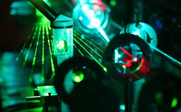
Born in the eighteenth century (Rittenhouse, 1786), the diffraction grating has been one of the most valuable instruments in the history of science and technology. At one extreme, it has enabled the study of celestial bodies. On the other hand, it has been a crucial tool in the study of atomic and molecular structures. These outstanding capabilities are the consequence of one basic property: it can disperse light, i.e. separate the frequencies contained in light radiation, thus allowing the measurement of relative intensities.

Grating description

Figure 1 represents a diffraction grating. The periodic profile \(\mathcal{P}\) of period along the -axis separates air from a grating material which is generally a metal or a dielectric. The -axis is perpendicular to the average profile plane and the -axis is the axis of invariance of the structure. We suppose that the incident light can be described by a sum of monochromatic radiations of different frequencies. Each of these can in turn be described in a time-harmonic regime, which allows us to use the complex notation (with an \(\exp(-i\omega t)\) time-dependence). The electromagnetic properties of the grating material (assumed to be non-magnetic) are represented by its complex refractive index \(\nu\) which depends on the wavelength \(\lambda=2\pi c/\omega\) in vacuum (\(c=1/\sqrt{\varepsilon_0\mu_0}\) being the speed of light, with \(\varepsilon_0\) and \(\mu_0\) the permittivity and the permeability of vacuum). This complex index respectively includes the conductivity (for metals) and/or the losses (for lossy dielectrics). It becomes a real number for lossless dielectrics.

In the air region, the grating is illuminated by an incident plane wave, assumed to be s-polarized (electric field parallel to the -axis) for simplicity, but the analysis is similar in the other case (p-polarization). With these conventions, the incident electric field \(\overrightarrow{E^i} =E^i\hat z\) (\(\hat z\) unit vector of the -axis) is given by \[\tag{1} E^i=\exp\bigl( ik_0 x\sin(\theta)-ik_0 y\cos(\theta)\bigr), \]

with \(\theta\) being the angle of incidence, from the -axis to the incident direction, measured in the counterclockwise sense, and \(k_0 = 2\pi/\lambda\) (we take an index equal to unity for air).

Plane wave expansion of the field, grating formula

Let us now introduce, without demonstration (Petit, 1980), three intuitive properties of the total electric field. Like the incident electric field \(\overrightarrow{E^i}\), the total field \(\overrightarrow{E}\) is:

• invariant along the -axis,
• parallel to the -axis, thus \(\overrightarrow{E}=E(x, y)\hat z\) .
• pseudo-periodic, i.e. by definition \[\tag{2} E(x+d, y)=E(x, y)\exp\bigl( ik_0 d\sin(\theta)\bigr) . \]

Notice that in normal incidence (\(\theta=0\) ), pseudo-periodicity becomes ordinary periodicity, which in that case is a straightforward property since both grating and incident wave are periodic.

Using these three properties and Maxwell's equations, let us show that the field above the grating is a sum of plane waves. With this aim, we use the first two Maxwell equations\[\tag{3} \nabla\times\overrightarrow{E}=i\omega\mu_0\overrightarrow{H}, \qquad \nabla\times\overrightarrow{H}=-i\omega\varepsilon\overrightarrow{E}, \]

with \(\overrightarrow{H}\) being the magnetic field and \(\varepsilon\) being the permittivity, equal to \(\varepsilon_0\) in air region and to \(\varepsilon_0 \nu^2\) in the grating material. In the following, equations placed at the left and right-hand sides of will be called first and second Maxwell equations respectively. Combining the two Maxwell equations the electric field satisfies in the entire space a Helmholtz equation\[\tag{4} \nabla^2E+k^2E=0, \]

with\[ k=\begin{cases}k_0 &\text{in the air} \\k_0 \nu &\text{in the material} \end{cases} \]

Moreover, it can be deduced from equation that \(E(x, y)\exp\bigl( -ik_0 x\sin(\theta)\bigr) \) has a period along the -axis and can thus be expanded in a Fourier series\[\tag{5} E(x, y)\exp\bigl( -ik_0 x\sin(\theta)\bigr) =\sum_{n=-\infty}^{+\infty} {E_n (y)\exp(2i\pi nx/d)}. \]

Multiplying both members of equation by \(\exp\bigl(ik_0 x\sin(\theta)\bigr)\) yields \[\tag{6} E(x, y)=\sum_{n=-\infty}^{+\infty} {E_n (y)\exp(i\alpha_n x)}, \qquad \alpha_n=k_0 \sin(\theta)+2\pi n/d. \]

Introducing this expression of \(E(x, y)\) in equation, we find \[\tag{7} \sum_{n=-\infty}^{+\infty}{\bigl( \mathrm{d^2}E_n (y)/\mathrm{d}y^2+\beta_n^2 E_n (y)\bigr) \exp(i\alpha_n x ) }=0, \qquad \beta_n=\sqrt{(k_0^2-\alpha_n^2)}. \]

Multiplying both members of the above equation by \(\exp\bigl (-ik_0 x\sin(\theta)\bigr) \), we obtain a Fourier series in the left-hand side. It is vital to bear in mind that the nullity of this Fourier series entails the nullity of its coefficients, provided that the Fourier series vanishes for any value of . Thus, equation must be satisfied for any value of . Since this equation is satisfied in the air region only, \(y\) must be greater than the ordinate \(y_M\) of the top of the grooves. In other words, we must restrict the property to the region located above the dotted blue line of figure 1. Finally, in this region\[\tag{8} \text{if } y>y_M, \qquad E_n(y)=I_n\exp(-i\beta_n y) + R_n\exp(+i\beta_n y), \]

and therefore, using equation, \(\tag{9} \text{if } y>y_M, \qquad E(x, y)=\sum_{n=-\infty}^{+\infty}{\bigl( I_n\exp(i\alpha_n x-i\beta_n y) + R_n\exp(i\alpha_n x+i\beta_n y)\bigr)}. \)